
By George Sterman,
Director of the C.N. Yang Institute for Theoretical Physics
Most of us would agree that addition and subtraction are simpler than multiplication and division, at least for big numbers. And this is not just for people who lack an affinity for math. When quantitative astronomy began in earnest, astronomers like Tycho Brahe and Johannes Kepler were faced with multiplications and divisions involving very large numbers, when they used trigonometry to deduce the motions of the planets. As seen in many other cases, this “practical” problem in the pursuit of pure science stimulated a solution with uses and implications far beyond its original inspiration. The unwieldy numbers of observational astronomy led to an innovation that reduced multiplication to addition, and division to subtraction. This invention was the logarithm, developed most influentially by John Napier around the beginning of the seventeenth century.
What are logarithms? Well, for every number “a” we define another number, log(a) , “the logarithm of a, ” which has the property that if c and d are two numbers, then the log of their product, log(cxd) is the sum of their two logarithms,
log (cxd) = log(c) + log(d).
How would this be used in practice? You have a table with a list of the (approximate) value of the logarithm for every positive number. Then, when presented with two large numbers with many digits, it’s not necessary to multiply them. Instead you go to that table of logs, look up the logs of the two numbers, add those two logs, and then return to the table to find out what number has that log. That new number will be the same as the product of the original numbers.
In days gone by, this property of logarithms was built into the scientific calculation tool of choice, the slide rule (see Figure 1).
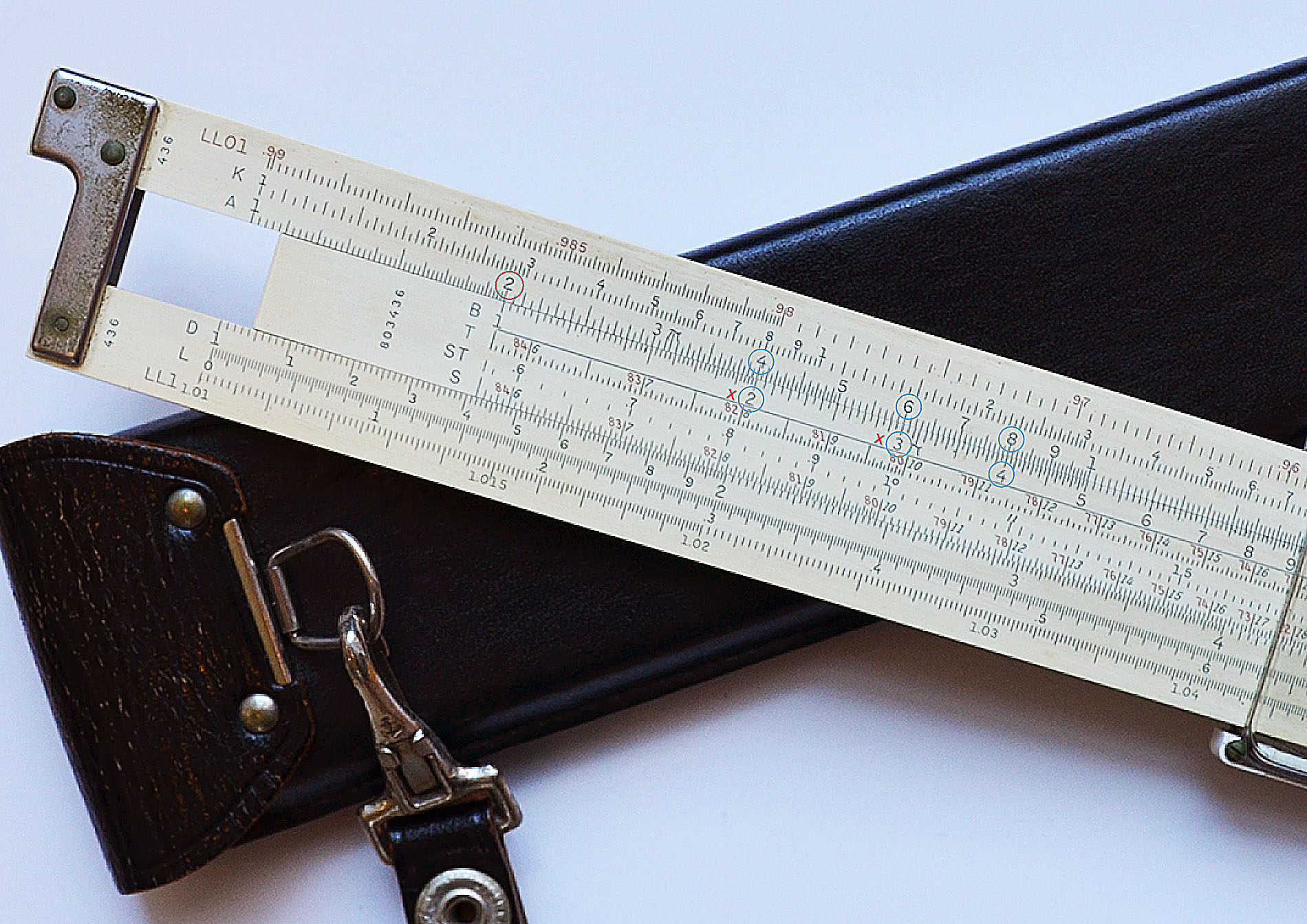
Figure 1. Slide rule. [From the office of C.N. Yang, Stony Brook University.]
A slide rule consists of two bars, one moveable (thus the name “slide”), with numbers marked out at points whose distances from the point marked 1 are proportional to their logarithms. Matching up the 1 on the moveable scale with any number X on the fixed scale does the multiplication of X times every number on the moveable scale automatically. From the figure, we check, for example, that 2 times 2 is 4 and 2 times 3 is 6, and so forth. Notice that in the picture the bigger numbers are getting closer together, which suggests that as the number N increases, log(N) doesn’t increase nearly as fast. To be specific, for large numbers, N, which means that 1/N is small,
log(N+1) = log(N) + log(1 + 1/N) ≈ log(N) + 1/N,
where the “wavy” equals sign means “approximately equal to.” We see that as we increase the number whose log we’re taking by 1, then to a very good approximation, the value of that logarithm increases only by 1/N. In fact, any time we identify a function f(x) that changes by 1/x when x changes by a unit, that function is proportional to log(x). [Note: here we are using what is called the “natural log.” There are other, equally good logarithms, but they are all found from the natural log by multiplying every natural log by the same number.]
Logarithms aren’t limited to their use in multiplication and division. They often occur in the description of natural phenomena, in quantities that change with distance, time, momentum or energy. But no matter how we measure these quantities, they can’t appear all by themselves in a logarithm, because you can find a log for the number 2, but not for 2 meters. A log can depend on a distance, but only if it is the distance measured in some unit, so that it is really the logarithm of a ratio, like
log (2 meters/1 meter).
But log(2 meters/1 meter) is the same number as log(2 miles/1 mile). Thus, if we change both the scale of the quantity (2 meters) and the scale of the unit of measure (1 meter) in the same way (meters to miles), we don’t change their ratio. We say that such a logarithm of a ratio is “scale invariant.” For most purposes a mile is very different than a meter, but in applications of the laws of nature, some measureable quantities can be scale invariant, at least approximately. In fact, scale invariance is a signal for the quantum field theories of the Standard Model. To see this, let’s talk about particles.
In the world of classical physics, we think of an isolated particle as stable in time. If the particle experiences a force, its motion will be changed, and Newton’s laws tell us just how this happens. Our classical particle knows about forces, but experiences them only if they are applied from the outside, or if the particle happens to move into a region where these forces act.
In the quantum view, things are much more lively. There is no such thing as a truly isolated particle. All quantum systems are restless — any particle will at all times experience all the forces to which it is sensitive, emitting and reabsorbing other particles that are associated with those forces. For electrons, the force is electromagnetism, and the associated particle is the photon. For quarks it’s the gluon of the strong interactions. This really means that a picture of nature in terms of isolated particles is inadequate, and that the “true” particles are more complex combinations of all these possibilities. Still, it’s convenient to think of an electron, for example, as emitting photons of specific energies, one at a time.
Such an emission changes the status quo, or “state,” consisting of a single electron to a new state, in which there is an electron and a photon. This state, however, has more energy than the original one. Classically, this forbids the whole process, because energy must be conserved, but in quantum mechanics such a state with the wrong energy can last for a finite amount of time, given on average by the ratio
T = (Planck’s constant) ⁄ (Photon’s energy).
So, an electron is never really alone, it always populates its neighborhood with such “virtual” photons, and we describe this situation as a “virtual state” of the electron.
Do virtual states really exist? Yes, we have good evidence that they do. Imagine that an electron in a virtual state is suddenly deflected by a force. For example, it might absorb a photon from another source. This can happen when our electron passes close by the nucleus of an atom. The process is illustrated in Figure 2, where the electron, represented by a straight line, comes in from the left, and emits a “virtual photon,” represented by a horizontal wavy line.
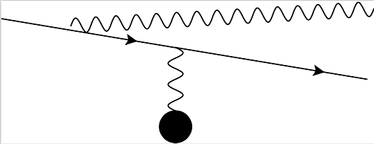
Figure 2. Feynman diagram for the Bethe-Heitler production of a photon.
Before it encounters the nucleus, the combination of the electron and photon doesn’t have the right energy to be “real.” (If it did, isolated electrons could emit photons, providing a kind of perpetual motion machine!). The energy is adjusted when the electron passes by the atomic nucleus, and the electron exchanges the other virtual photon (the vertical wavy line) with the nucleus (the black circle), so that both the virtual photon and the electron now have just the right energy for their momenta, and off they both go on the right of the figure, in a state that can last indefinitely. When this happens, the process is called the “Bethe-Heitler” production of a photon. This is basically how X-rays are produced for medical imaging and other purposes.
In the Bethe-Heitler process, the nucleus in effect “shakes loose” the photon from the electron, and the two separate, as would any other virtual partners that happened to be “in the air” of the particular virtual state at the particular time the electron passes by the nucleus. A photon is, however, by far the most likely virtual partner, because it can carry just a little energy, thus occurring in virtual states that can last a long time.
A picture like Figure 2 is sometimes referred to as a “Feynman diagram,” which illustrates quantum-mechanical processes like this one. These diagrams help us picture such quantum processes intuitively, and they also come with rules that tell us how to turn the intuitive picture into quantitative predictions. How likely is the Bethe-Heitler process, and how does it depend on the energy of the virtual state? This depends on the theory and on the energy transfer. The rules for Feynman diagrams in each theory are used to compute the answers.
Famously, quantum mechanics makes predictions in terms of probabilities, numbers that have to be somewhere between 0 and 1, where 1 indicates “a sure thing” and 0, “not a chance.”
The probabilities that tell us how elementary particles behave in isolation or in collisions actually depend on the number of dimensions in our world, because whatever its energy, the virtual photon could move in any direction, and the range of possible directions depends on how many dimensions there are. This is where the logarithms come in. When we calculate the probability of finding an electron in a state with a photon of energy E, summing over all directions in three space like 1/E, the telltale sign that the total probability is a log. The same goes for finding a quark accompanied by a gluon, in the theory of the strong interactions that is part of the Standard Model.
This 1/E dependence means that the total probability for the Bethe-Heitler production of photons between any two energies is given by the logarithm of the ratio of those energies. Suppose, then, we ask for the probability for encountering photons in a range of energies, say from Emin to Emax. For a single photon the answer is of the form
Probability to find one photon = F x α2 log (Emax/Emin),
where F depends on the velocity and direction of the electron before and after the collision, and α is a number called the “electromagnetic coupling.” It is a measure of how easily virtual states change one into another. It is one of the fundamental constants in nature. Its value is small, about 1/137. It is a “pure number” with no units, and if it were not, the energy dependence would have been different.
The Bethe-Heitler logarithm exhibits the property of scale invariance — if we multiply the smaller and larger scales by the same number, we get the same probability. The probability of finding a photon emitted between (say) 2 electron volts and 4 electron volts is the same as between 4 electron volts and 8 electron volts. This feature also appears, at least approximately, at much higher energies for all the components of contemporary particle physics, that is, the Standard Model. Approximate scale invariance is a direct result of having dimensionless coupling constants and of being in four dimensions (three space, one time).
So far so good, but there is a surprising consequence of this picture. After all, the electron isn’t always so unfortunate as to pass by a nucleus while its photon companion, of energy E, is in a virtual state. Left undisturbed, after a time proportional to 1/E, the electron reunites with its virtual friend. But using just the same method, we can calculate the probability for all such “unseen” photons between two energies, Emin and Emax, to be emitted and then absorbed. When we do, we get the same log(Emax/Emin), as in the Bethe-Heitler process. But if we don’t see these virtual photons, there really is no limit to their maximum energy, Emax, and we end up with the logarithm of infinity, which is itself infinite. This is a property shared by all the quantum field theories in the Standard Model; they all have infinities, which emerge through logarithms, from the hidden lives of their elementary particles. In effect, the electrons of the Standard Model are spendthrift with energy, loaning it freely to their virtual photons with no limit. And yet, these loans are always repaid. Technically, this problem is avoided by a method known as “renormalization,” which can be applied successfully to theories with dimensionless couplings. Renormalization “hides” whatever it is that keeps virtual photons from carrying infinite energies to and from their parent electrons.
After renormalization, approximate scale invariance has a tendency to isolate low energy phenomena from the influence of whatever lies at higher energies or shorter distances. In fact, the Standard Model may turn out to be difficult to improve upon, simply because its approximate scale invariance makes its predictions self-consistent up to energies far beyond those directly accessible to accelerators. The emphasis here is on the word “may,” because this scale invariance may fail past a certain energy, indicating the presence of new fixed energy scales beyond those we know today.
Einstein felt that dimensionless constants ought not to be a basic ingredient in a truly fundamental theory[1], and over the years the logarithmic infinities associated with them have displeased many illustrious physicists. The very first natural force law, of Newton’s gravity, is defined with a dimension- full number, known as “Newton’s constant.” The most influential modern “completion” of the Standard Model including gravity is string theory, in which the basic constant is the string tension, a quantity with dimensions, related to Newton’s constant. The logarithms at the heart of the Standard Model may yet yield to compelling experimental or theoretical evidence for new, dimensional scales that can tell a meter from a mile, or a gram from a ton.
[1] Ilse Rosenthal-Schneider, “Reality and Scientific Truth: Discussions with Einstein, Von Laue, and Planck.” Wayne State University Press (1980), pp. 36, 41 and 74.